Phenotypic selection analysis in R

I have up to recently always done my phenotypic selection analyses in SAS. I finally got some code I think works to do everything SAS would do. Feedback much appreciated!

########################Selection analyses#############################
install.packages(c("car","reshape","ggplot2"))
require(car)
require(reshape)
require(ggplot2)
 
# Create data set
dat <- data.frame(plant = seq(1,100,1),
 trait1 = rep(c(0.1,0.15,0.2,0.21,0.25,0.3,0.5,0.6,0.8,0.9,1,3,4,10,11,12,13,14,15,16), each = 5), trait2 = runif(100),
 fitness = rep(c(1,5,10,20,50), each = 20))
 
# Make relative fitness column
dat_ <- cbind(dat, dat$fitness/mean(dat$fitness))
names(dat_)[5] <- "relfitness"
 
# Standardize traits
dat_ <- cbind(dat_[,-c(2:3)], rescaler(dat_[,c(2:3)],"sd"))
 
####Selection differentials and correlations among traits, cor.prob uses function in functions.R file
############################################################################
####### Function for calculating correlation matrix, corrs below diagonal,
####### and P-values above diagonal
############################################################################
cor.prob <- function(X, dfr = nrow(X) - 2) {
         R <- cor(X)
         above <- row(R) < col(R)
         r2 <- R[above]^2
         Fstat <- r2 * dfr / (1 - r2)
         R[above] <- 1 - pf(Fstat, 1, dfr)
         R
} 
 
# Get selection differentials and correlations among traits in one data frame
dat_seldiffs <- cov(dat_[,c(3:5)]) # calculates sel'n differentials using cov
dat_selcorrs <- cor.prob(dat_[,c(3:5)]) # use P-values above diagonal for significance of sel'n differentials in dat_seldiffs
dat_seldiffs_selcorrs <- data.frame(dat_seldiffs, dat_selcorrs) # combine the two
 
##########################################################################
####Selection gradients
dat_selngrad <- lm(relfitness ~ trait1 * trait2, data = dat_)
summary(dat_selngrad) # where "Estimate" is our sel'n gradient
 
####Check assumptions
shapiro.test(dat_selngrad$residuals) # normality, bummer, non-normal
hist(dat_selngrad$residuals) # plot residuals
vif(dat_selngrad) # check variance inflation factors (need package car), everything looks fine
plot(dat_selngrad) # cycle through diagnostic plots
 
############################################################################
# Plot data
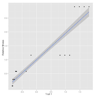
ggplot(dat_, aes(trait1, relfitness)) +
 geom_point() +
 geom_smooth(method = "lm") +
 labs(x="Trait 1",y="Relative fitness")
ggsave("myplot.jpeg")

Created by Pretty R at inside-R.org


Plot of relative fitness vs. trait 1 standardized