Weecology can has new mammal dataset

Recology has moved - go to http://recology.info/2011/12/weecology-can-has-new-mammal-dataset

So the Weecology folks have published a large dataset on mammal communities in a data paper in Ecology.  I know nothing about mammal communities, but that doesn't mean one can't play with the data...

Their dataset consists of five csv files:  communities, references, sites, species, and trapping data.

Where are these sites, and by the way, do they vary much in altitude?

Let's zoom in on just 'the states'?



What phylogenies can we get for the species in this dataset?
We can use the rOpenSci package treebase to search the online phylogeny repository TreeBASE.  Limiting to returning a max of 1 tree (to save time), we can see that X species are in at least 1 tree on the TreeBASE database.  Nice. 

So there are 321 species in the database with at least 1 tree in the TreeBASE database.  Of course there could be many more, but we limited results from TreeBASE to just 1 tree per query. 

Here's the code:

I Work For The Internet !

Recology has moved, go to http://recology.info/2011/12/i-work-for-internet

UPDATE: code and figure updated at 647 AM CST on 19 Dec '11.  Also, see Jarrett Byrnes (improved) fork of my gist  here.


The site I WORK FOR THE INTERNET is collecting pictures and first names (last name initials only) to show collective support against SOPA (the Stop Online Piracy Act).  Please stop by their site and add your name/picture.

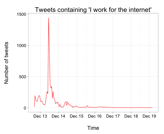
I used the #rstats package twitteR, created by Jeff Gentry, to search for tweets from people signing this site with their picture, then plotted using ggplot2, and also used Hadley's lubridate to round timestamps on tweets to be able to bin tweets in to time slots for plotting.

Tweets containing the phrase 'I work for the internet' by time:

Here's the code as a GitHub gist.   Sometimes the searchTwitter fxn doesn't returns an error, which I don't understand, but you can play with it:

ggplot2 talk by Hadley Whickam at Google

plyr's idata.frame VS. data.frame

I had seen the function idata.frame in plyr before, but not really tested it. From the plyr documentation:

"An immutable data frame works like an ordinary data frame, except that when you subset it, it
returns a reference to the original data frame, not a a copy. This makes subsetting substantially
faster and has a big impact when you are working with large datasets with many groups."

For example, although baseball is a data.frame, its immutable counterpart is a reference to it:

> idata.frame(baseball)
<environment: 0x1022c74e8>
attr(,"class")
[1] "idf"         "environment"

Here are a few comparisons of operations on normal data frames and immutable data frames. Immutable data frames don't work with the doBy package, but do work with aggregate in base functions.  Overall, the speed gains using idata.frame are quite impressive - I will use it more often for sure.


Get the github code below here.





Here's the comparisons of idata.frames and data.frames:

> # load packages
require(plyr); require(reshape2)
 
> # Make immutable data frame
baseball_i <- idata.frame(baseball)
 
> # Example 1 - idata.frame more than twice as fast
system.time( replicate(50, ddply( baseball, "year", summarise, mean(rbi))) )
   user  system elapsed 
 14.812   0.252  15.065 
> system.time( replicate(50, ddply( baseball_i, "year", summarise, mean(rbi))) )
   user  system elapsed 
  6.895   0.020   6.915 

> # Example 2 - Bummer, this does not work with idata.frame's> colwise(max, is.numeric) ( baseball ) # works
  year stint   g  ab   r   h X2b X3b hr rbi sb cs  bb so ibb hbp sh sf gidp
1 2007     4 165 705 177 257  64  28 73  NA NA NA 232 NA  NA  NA NA NA   NA
> colwise(max, is.numeric) ( baseball_i ) # doesn't work
Error: is.data.frame(df) is not TRUE

> # Example 3 - idata.frame twice as fast
system.time( replicate(100, baseball[baseball$year == "1884", ] ) )
   user  system elapsed 
  1.155   0.048   1.203 
> system.time( replicate(100, baseball_i[baseball_i$year == "1884", ] ) )
   user  system elapsed 
  0.598   0.011   0.609 

> # Example 4 - idata.frame faster
system.time( replicate(50, melt(baseball[, 1:4], id = 1) ) )
   user  system elapsed 
 16.587   1.169  17.755 
> system.time( replicate(50, melt(baseball_i[, 1:4], id = 1) ) )
   user  system elapsed 
  0.869   0.196   1.065 

> # And you can go back to a data frame by 
d <- as.data.frame(baseball_i)
str(d)
 
'data.frame': 21699 obs. of  23 variables:
 $ id   : chr  "ansonca01" "forceda01" "mathebo01" "startjo01" ...
 $ year : int  1871 1871 1871 1871 1871 1871 1871 1872 1872 1872 ...
 $ stint: int  1 1 1 1 1 1 1 1 1 1 ...
 $ team : chr  "RC1" "WS3" "FW1" "NY2" ...
 $ lg   : chr  "" "" "" "" ...
 $ g    : int  25 32 19 33 29 29 29 46 37 25 ...
 $ ab   : int  120 162 89 161 128 146 145 217 174 130 ...
 $ r    : int  29 45 15 35 35 40 36 60 26 40 ...
 $ h    : int  39 45 24 58 45 47 37 90 46 53 ...
 $ X2b  : int  11 9 3 5 3 6 5 10 3 11 ...
 $ X3b  : int  3 4 1 1 7 5 7 7 0 0 ...
 $ hr   : int  0 0 0 1 3 1 2 0 0 0 ...
 $ rbi  : int  16 29 10 34 23 21 23 50 15 16 ...
 $ sb   : int  6 8 2 4 3 2 2 6 0 2 ...
 $ cs   : int  2 0 1 2 1 2 2 6 1 2 ...
 $ bb   : int  2 4 2 3 1 4 9 16 1 1 ...
 $ so   : int  1 0 0 0 0 1 1 3 1 0 ...
 $ ibb  : int  NA NA NA NA NA NA NA NA NA NA ...
 $ hbp  : int  NA NA NA NA NA NA NA NA NA NA ...
 $ sh   : int  NA NA NA NA NA NA NA NA NA NA ...
 $ sf   : int  NA NA NA NA NA NA NA NA NA NA ...
 $ gidp : int  NA NA NA NA NA NA NA NA NA NA ...
 $ teamf: Factor w/ 132 levels "ALT","ANA","ARI",..: 99 127 51 79 35 35 122 86 16 122 ...

> # idata.frame doesn't work with the doBy package
require(doBy)
summaryBy(rbi ~ year, baseball_i, FUN=c(mean), na.rm=T)
Error in as.vector(x, mode) : 
  cannot coerce type 'environment' to vector of type 'any'

> # But idata.frame works with aggregate in base (but with minimal speed gains)
# and aggregate is faster than ddply of course 
system.time( replicate(100, aggregate(rbi ~ year, baseball, mean) ) )
   user  system elapsed 
  4.117   0.423   4.541 
> system.time( replicate(100, aggregate(rbi ~ year, baseball_i, mean) ) )
   user  system elapsed 
  3.908   0.383   4.291 
> system.time( replicate(100, ddply( baseball_i, "year", summarise, mean(rbi)) ) )
   user  system elapsed 
 14.015   0.048  14.082 

Created by Pretty R at inside-R.org

Troubling news for the teaching of evolution

[UPDATE: i remade the maps in green, hope that helps...]

A recent survey reported in Science ("Defeating Creationism in the Courtroom, but not in the Classroom") found that biology teachers in high school do not often accept the basis of their discipline, as do teachers in other disciplines, and thus may not teach evolution appropriately. Read more here: New York Times.

I took a little time to play with the data provided online along with the Science article. The data is available on the Science website along with the article, and the dataset I read into R is unchanged from the original. The states abbreviations file is here (as a .xls). Here goes:

I only played with two survey questions: q1b (no. of hours ecology is taught per year), and q1d (no. of hours evolution is taught per year). I looked at ecology and evolution as this blog is about ecology and evolution. It seems that some states that teach a lot of ecology teach a lot of evolution, but I found no correlation between the two without extreme outliers. I couldn’t help but notice my home state, TX, is near the bottom of the list on both counts - go TX! The teaching of evolution on the map produced below is less predictable than I would have though just based on my assumptions about political will in each state.

# Analyses of Conditionality Data set of all variables, except for latitude, etc.
setwd("/Mac/R_stuff/Blog_etc/EvolutionTeaching/") # Set working directory
library(ggplot2)
 
# read in data, and prepare new columns
survey <- read.csv("berkmandata.csv")
str(survey) # (I do realize that survey is a data object in the MASS package)
 
# Assign actual hours to survey answers 
ecol <- gsub(1, 0, survey$q1b)
ecol <- gsub(2, 1.5, ecol)
ecol <- gsub(3, 4, ecol)
ecol <- gsub(4, 8, ecol)
ecol <- gsub(5, 13, ecol)
ecol <- gsub(6, 18, ecol)
ecol <- gsub(7, 20, ecol)
 
evol <- gsub(1, 0, survey$q1d)
evol <- gsub(2, 1.5, evol)
evol <- gsub(3, 4, evol)
evol <- gsub(4, 8, evol)
evol <- gsub(5, 13, evol)
evol <- gsub(6, 18, evol)
evol <- gsub(7, 20, evol)
 
survey$ecol <- as.numeric(ecol)
survey$evol <- as.numeric(evol)
 
# ddply it
survey_sum <- ddply(survey, .(st_posta), summarise,
 mean_ecol_hrs = mean(ecol, na.rm=T),
 mean_evol_hrs = mean(evol, na.rm=T),
 se_ecol_hrs = sd(ecol, na.rm=T)/sqrt(length(ecol)),
 se_evol_hrs = sd(evol, na.rm=T)/sqrt(length(evol)),
 num_teachers = length(st_posta)
)
 
# plotting
limits_ecol <- aes(ymax = mean_ecol_hrs + se_ecol_hrs, ymin = mean_ecol_hrs - se_ecol_hrs)
limits_evol <- aes(ymax = mean_evol_hrs + se_evol_hrs, ymin = mean_evol_hrs - se_evol_hrs)
 
ggplot(survey_sum, aes(x = reorder(st_posta, mean_ecol_hrs), y = mean_ecol_hrs)) +
 geom_point() +
 geom_errorbar(limits_ecol) +
 geom_text(aes(label = num_teachers), vjust = 1, hjust = -3, size = 3) +
 coord_flip() +
 labs(x = "State", y = "Mean hours of ecology taught \n per year (+/- 1 se)")

####SMALL NUMBERS BY BARS ARE NUMBER OF TEACHERS THAT RESPONDED TO THE SURVEY

 
ggplot(survey_sum, aes(x = reorder(st_posta, mean_evol_hrs), y = mean_evol_hrs)) +
 geom_point() +
 geom_errorbar(limits_evol) +
 geom_text(aes(label = num_teachers), vjust = 1, hjust = -3, size = 3) +
 coord_flip() +
 labs(x = "State", y = "Mean hours of evolution taught \n per year (+/- 1 se)")
 ####SMALL NUMBERS BY BARS ARE NUMBER OF TEACHERS THAT RESPONDED TO THE SURVEY


 
# map
try_require("maps")
states <- map_data("state")
statenames <- read.csv("/Mac/R_stuff/Code/states_abbreviations.csv")
survey_sum_ <- merge(survey_sum, statenames, by.x = "st_posta", by.y = "state_abbrev")
survey_sum_map <- merge(states, survey_sum_, by.x = "region", by.y = "state")
survey_sum_map <- survey_sum_map[order(survey_sum_map$order), ]
 
qplot(long, lat, data = survey_sum_map, group = group, fill = mean_ecol_hrs, geom = "polygon") + scale_fill_gradient(low="black", high="green")

 

qplot(long, lat, data = survey_sum_map, group = group, fill = mean_evol_hrs, geom = "polygon") + scale_fill_gradient(low="black", high="green")

Created by Pretty R at inside-R.org

Good riddance to Excel pivot tables

Excel pivot tables have been how I have reorganized data...up until now. These are just a couple of examples why R is superior to Excel for reorganizing data:

UPDATE: I fixed the code to use 'dcast' instead of 'cast'. And library(ggplot2) instead of library(plyr) [plyr is called along with ggplot2]. Thanks Bob!

Also, see another post on this topic:
-http://news.mrdwab.com/2010/08/08/using-the-reshape-packagein-r/

################ Good riddance to pivot tables ############
library(reshape2)
library(ggplot2) 
dataset <- data.frame(var1 = rep(c("a","b","c","d","e","f"), each = 4), 
 var2 = rep(c("level1","level1","level2","level2"), 6), 
 var3 = rep(c("h","m"), 12), meas = rep(1:12))

Created by Pretty R at inside-R.org

# simply pivot table
dcast(dataset, var1 ~ var2 + var3)
Using meas as value column.  Use the value argument to cast to override this choice
  var1 level1_h level1_m level2_h level2_m
1    a        1        2        3        4
2    b        5        6        7        8
3    c        9       10       11       12
4    d        1        2        3        4
5    e        5        6        7        8
6    f        9       10       11       12

 
# mean by var1 and var2
dcast(dataset, var1 ~ var2, mean)

Using meas as value column.  Use the value argument to cast to override this choice
  var1 level1 level2
1    a    1.5    3.5
2    b    5.5    7.5
3    c    9.5   11.5
4    d    1.5    3.5
5    e    5.5    7.5
6    f    9.5   11.5

 
# mean by var1 and var3
dcast(dataset, var1 ~ var3, mean)
Using meas as value column.  Use the value argument to cast to override this choice
  var1  h  m
1    a  2  3
2    b  6  7
3    c 10 11
4    d  2  3
5    e  6  7
6    f 10 11

 
# mean by var1, var2 and var3 (version 1)
dcast(dataset, var1 ~ var2 + var3, mean)

Using meas as value column.  Use the value argument to cast to override this choice
  var1 level1_h level1_m level2_h level2_m
1    a        1        2        3        4
2    b        5        6        7        8
3    c        9       10       11       12
4    d        1        2        3        4
5    e        5        6        7        8
6    f        9       10       11       12
 
# mean by var1, var2 and var3 (version 2)
dcast(dataset, var1 + var2 ~ var3, mean)

Using meas as value column.  Use the value argument to cast to override this choice
   var1   var2  h  m
1     a level1  1  2
2     a level2  3  4
3     b level1  5  6
4     b level2  7  8
5     c level1  9 10
6     c level2 11 12
7     d level1  1  2
8     d level2  3  4
9     e level1  5  6
10    e level2  7  8
11    f level1  9 10
12    f level2 11 12

 
# use package plyr to create flexible data frames...
dataset_plyr <- ddply(dataset, .(var1, var2), summarise, 
 mean = mean(meas), 
 se = sd(meas),
 CV = sd(meas)/mean(meas)
)
> dataset_plyr
   var1   var2 mean        se         CV
1     a level1  1.5 0.7071068 0.47140452
2     a level2  3.5 0.7071068 0.20203051
3     b level1  5.5 0.7071068 0.12856487
4     b level2  7.5 0.7071068 0.09428090
5     c level1  9.5 0.7071068 0.07443229
6     c level2 11.5 0.7071068 0.06148755
7     d level1  1.5 0.7071068 0.47140452
8     d level2  3.5 0.7071068 0.20203051
9     e level1  5.5 0.7071068 0.12856487
10    e level2  7.5 0.7071068 0.09428090
11    f level1  9.5 0.7071068 0.07443229
12    f level2 11.5 0.7071068 0.06148755

 
# ...to use for plotting
qplot(var1, mean, colour = var2, size = CV, data = dataset_plyr, geom = "point")

Created by Pretty R at inside-R.org