Weecology can has new mammal dataset

Recology has moved - go to http://recology.info/2011/12/weecology-can-has-new-mammal-dataset

So the Weecology folks have published a large dataset on mammal communities in a data paper in Ecology.  I know nothing about mammal communities, but that doesn't mean one can't play with the data...

Their dataset consists of five csv files:  communities, references, sites, species, and trapping data.

Where are these sites, and by the way, do they vary much in altitude?

Let's zoom in on just 'the states'?



What phylogenies can we get for the species in this dataset?
We can use the rOpenSci package treebase to search the online phylogeny repository TreeBASE.  Limiting to returning a max of 1 tree (to save time), we can see that X species are in at least 1 tree on the TreeBASE database.  Nice. 

So there are 321 species in the database with at least 1 tree in the TreeBASE database.  Of course there could be many more, but we limited results from TreeBASE to just 1 tree per query. 

Here's the code:

My little presentation on getting web data through R

Recology has moved, go to http://recology.info/my-little-presentation-on-getting-web
With examples from rOpenSci R packages. p.s. I am no expert at this...
Web data from R

View more presentations from schamber

rnpn: An R interface for the National Phenology Network

Recology has moved, go to http://recology.info/2011/08/rnpn-r-interface-for-national-phenology

The team at rOpenSci and I have been working on a wrapper for the USA National Phenology Network API. The following is a demo of some of the current possibilities. We will have more functions down the road. Get the publicly available code, and contribute, at Github here. If you try this out look at the Description file for the required R packages to run rnpn. Let us know at Github (here) or at our website  http://ropensci.org/, or in the comments below, or on twitter (@rOpenSci), what use cases you would like to see with the rnpn package.

Method and demo of each:
Get observations for species by day
From the documentation: "This function will return a list of species, containing all the dates which observations were made about the species, and a count of the number of such observations made on that date."

#### Note, the data below is truncated for blogging brevity...

> getobsspbyday(c(1, 2), '2008-01-01', '2011-12-31') # Searched for species 1 and 2 from Jan 1, 2008 to Dec 31, 2011
          date count   species
1   2009-03-08     2 species 1
2   2009-03-15     1 species 1
3   2009-03-22     1 species 1
4   2009-03-24     1 species 1
5   2009-03-26     1 species 1
6   2009-04-17     1 species 1
7   2009-04-24     1 species 1
8   2009-05-12     1 species 1
9   2009-05-20     1 species 1
10  2009-11-24     1 species 1
11  2009-12-07     1 species 1
12  2010-01-18     1 species 1
13  2010-01-23     1 species 1
62  2011-05-29     1 species 1
63  2011-06-27     1 species 1
64  2011-06-30     2 species 1
65  2009-03-17     1 species 2
66  2009-04-03     3 species 2
67  2009-04-05     3 species 2
68  2009-04-10     3 species 2
69  2009-04-17     3 species 2

Get individuals at specific stations
From the documentation: "This function returns all of the individuals at a series of stations."

> getindsatstations(c(507, 523)) # Searched for any individuals at stations 507 and 523
   individual_id individual_name species_id kingdom
1           1200         dogwood         12 Plantae
2           1197    purple lilac         36 Plantae
3           1193         white t         38 Plantae
4           3569     forsythia-1         73 Plantae
5           1206            jack        150 Plantae
6           1199      trout lily        161 Plantae
7           1198           dandy        189 Plantae
8           1192           red t        192 Plantae
9           1710    common lilac         36 Plantae
10          1711  common lilac 2         36 Plantae
11          1712       dandelion        189 Plantae

Get individuals of species at stations
From the documentation: "This function will return a list of all the individuals, which are members of a species, among  any number of stations."

> getindspatstations(35, c(60, 259), 2009)  # Search for individuals of species 35 at stations 60 and 259 in year 2009
  individual_id individual_name number_observations
1          1715            west                   5
2          1716            east                   5

Get observation associated with particular observation
From the documentation: "This function will return the comment associated with a particular observation."

> getobscomm(1938) # The observation for observation number 1938

$observation_comment
[1] "some lower branches are bare"

(#ESA11) rOpenSci: a collaborative effort to develop R-based tools for facilitating Open Science

Recology has moved, go to http://recology.info/2011/08/esa11-ropensci-collaborative-effort-to_08

Our development team would like to announce the launch of rOpenSci. As the title states, this project aims to create R packages to make open science more available to researchers.

http://ropensci.org/

What this means is that we seek to connect researchers using R with as much open data as possible, mainly through APIs. There are a number of R packages that already do this (e.g., infochimps, twitteR), but we are making more packages, e.g., for Mendeley, PLoS Journals, and taxonomic sources (ITIS, EOL, TNRS, Phylomatic, UBio).

Importantly, we are creating a package called rOpenSci, which aims to integrate functions from packages for individual open data sources.

If you are somewhat interested, follow our progress on our website, on Twitter, or contact us. If you are really^2 interested you could go to Github and contribute. If  you are really^3 interested, join our development team.

Archiving ecology/evolution data sets online

We now have many options for archiving data sets online:

Dryad, KNB, Ecological Archives, Ecology Data Papers, Ecological Data, etc.

However, these portals largely do not communicate with one another as far as I know, and there is no way to search over all data set sources, again, as far as I know. So, I wonder if it would ease finding of all these different data sets to get these different sites to get their data sets cloned on a site like Infochimps, or have links from Infochimps.  Infochimps already has APIs (and there's an R wrapper for the Infochimps API already set up here: http://cran.r-project.org/web/packages/infochimps/index.html by Drew Conway), and they have discussions set up there, etc.

Does it make sense to post data sets linked to published works on Infochimps? I think probably not know that I think about it. But perhaps it makes sense for other data sets, or subsets of data sets that are not linked with published works to be posted there as I know at least Dryad only accepts data sets linked with published papers.

One use case is there was a tweet from someone recently that his students were excited about getting their data sets on their resume/CV, but didn't think there was a way to put them any place where there wasn't a precondition that the data set was linked with a published work. Seems like this could be a good opportunity to place these datasets on Infcohimps, and at least they are available then where a lot of people are searching for data sets, etc.

What I think would be ideal is if Dryad, KNB, etc. could link their datasets to Infochimps, where they could be found, then users can either get them from Infochimps, or perhaps you would have to go to the Dryad site, e.g. But at least you could search over all ecological data sets then.

rbold: An R Interface for Bold Systems barcode repository

Have you ever wanted to search and fetch barcode data from Bold Systems?

I am developing functions to interface with Bold from R. I just started, but hopefully folks will find it useful.

The code is at Github here. The two functions are still very buggy, so please bring up issues below, or in the Issues area on Github. For example, some searches work and other similar searches don't. Apologies in advance for the bugs.

Below is a screenshot of an example query using function getsampleids to get barcode identifiers for specimens. You can then use getseqs function to grab barcode data for specific specimens or many specimens.

iEvoBio 2011 Synopsis

We just wrapped up the 2011 iEvoBio meeting. It was awesome! If you didn't go this year or last year, definitely think about going next year.

Here is a list of the cool projects that were discussed at the meeting (apologies if I left some out):

1. Vistrails: workflow tool, awesome project by Claudio Silva
2. Commplish: purpose is to use via API's, not with the web UI
3. Phylopic: a database of life-form silouhettes, including an API for remote access, sweet!
4. Gloome
5. MappingLife: awesome geographic/etc data visualization interace on the web
6. SuiteSMA: visualizating multiple alignments
7. treeBASE: R interface to treebase, by Carl Boettiger
8. VertNet: database for vertebrate natural history collections
9. RevBayes: revamp of MrBayes, with GUI, etc. 
10. Phenoscape Knowledge Base
• Peter Midford lightning talk: talked about matching taxonomic and genetic data
11. BiSciCol: biological science collections tracker
12. Ontogrator 
13. TNRS: taxonomic name resolution service
14. Barcode of Life data systems, and remote access
15. Moorea Biocode Project
16. Microbial LTER's data
17. BirdVis: interactive bird data visualization (Claudio Silva in collaboration with Cornell Lab of Ornithology)
18. Crowdlabs: I think the site is down right now, another project by Claudio Silva
19. Phycas: Bayesian phylogenetics, can you just call this from R?
20. RIP MrBayes!!!! replaced by RevBayes (see 9 above)
21. Slides of presentations will be at Slideshare (not all presentations up yet)          
22. A birds of a feather group I was involved in proposed an idea (TOL-o-matic) like Phylomatic, but of broader scope, for easy access and submission of trees, and perhaps even social (think just pushing a 'SHARE' button within PAUP, RevBayes, or other phylogenetics software)! 
23. Synopses of Birds of a Feather discussion groups: http://piratepad.net/iEvoBio11-BoF-reportouts

OpenStates from R via API: watch your elected representatives

I am writing some functions to acquire data from the OpenStates project, via their API. They have a great support community at Google Groups as well.

On its face this post is not obviously about ecology or evolution, but well, our elected representatives do, so to speak, hold our environment in a noose, ready to let the Earth hang any day.

Code I am developing is over at Github.

Here is an example of its use in R, in this case using the Bill Search option (billsearch.R on my Github site), and in this case you do not provide your API key in the function call, but instead put it in your .Rprofile file, which is called when you open R. We are searching here for the term 'agriculture' in Texas ('tx'), in the 'upper' chamber.

> temp <- billsearch('agriculture', state = 'tx', chamber = 'upper')
 
> length(temp)
[1] 21
 
> temp[[1]]
$title
[1] "Congratulating John C. Padalino of El Paso for being appointed to the United States Department of Agriculture."
 
$created_at
[1] "2010-08-11 07:59:46"
 
$updated_at
[1] "2010-09-02 03:34:39"
 
$chamber
[1] "upper"
 
$state
[1] "tx"
 
$session
[1] "81"
 
$type
$type[[1]]
[1] "resolution"
 
 
$subjects
$subjects[[1]]
[1] "Resolutions"
 
$subjects[[2]]
[1] "Other"
 
 
$bill_id
[1] "SR 1042"

Created by Pretty R at inside-R.org


Apparently, the first bill (SR 2042, see $bill_id at the bottom of the list output) that came up was to congratulate John Paladino for being appointed to the USDA.

The other function I have ready is getting basic metadata on a state, called statemetasearch.

I plan to develop more functions for all the possible API calls to the OpenStates project.

Farmer's markets data

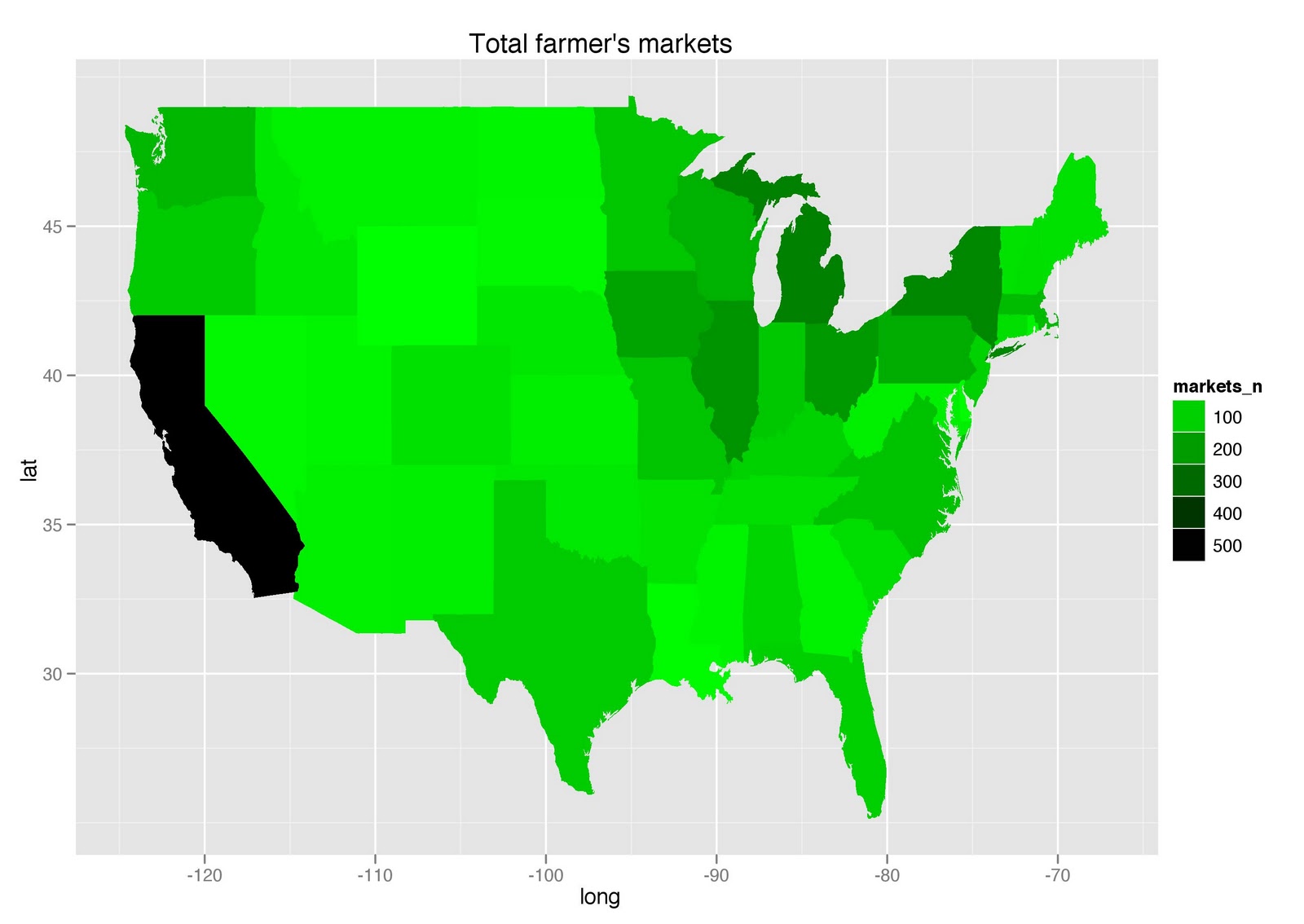
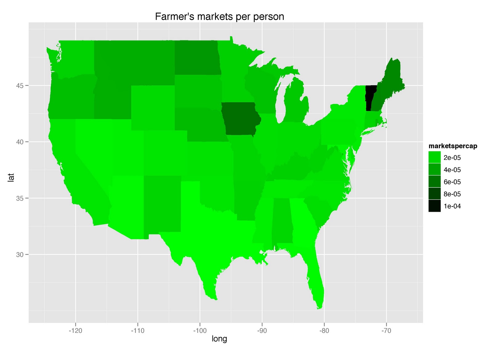
I combined USDA data on farmer's markets in the US with population census data to get an idea of the disparity in farmers markets by state, and then also expressed per capita.

Download USDA data here. The formatted file I used below is here (in excel format, although I read into R as csv file). The census data is read from url as below.

California has a ton of absolute number of farmer's markets, but Vermont takes the cake by far with number of markets per capita. Iowa comes in a distant second behind Vermont in markets per capita.



The code:

######## Farmer's Markets #############
setwd("/Mac/R_stuff/Blog_etc/USDAFarmersMarkets") # Set to your working directory, this is where you want to call files from and write files to
install.packages(c("ggplot2", "RCurl"))  # install all packags required below
require(ggplot2) # plyr is libraried along with ggplot2, as ggplot2 uses plyr (as well as package reshape) functions
 
# read market data
markets <- read.csv("farmmarkets.csv")
markets$state <- as.factor(gsub("Wyoming ", "Wyoming", markets$LocAddState)) # there was a typo for Wyoming
markets <- na.omit(markets)
str(markets)
 
# read population census data
popcen <- read.csv("http://www.census.gov/popest/national/files/NST_EST2009_ALLDATA.csv")
popcen <- popcen[,c(4,5,6,17)]
str(popcen)
 
# summarize
markets_ <- ddply(markets, .(state), summarise,
 markets_n = length(LocAddState) 
)
 
markets_pop_ <- merge(markets_, popcen[,-1], by.x = "state", by.y = "NAME") # merge two data sets
markets_pop_$marketspercap <- markets_pop_$markets_n/markets_pop_$POPESTIMATE2009 # create column of markets per capita
markets_pop_$markets_n_st <- markets_pop_$markets_n/max(markets_pop_$markets_n)
markets_pop_$marketspercap_st <- markets_pop_$marketspercap/max(markets_pop_$marketspercap)
 
# plot
ggplot(melt(markets_pop_[,-c(2:5)]), aes(x = state, y = value, fill = variable)) +
 geom_bar(position = "dodge") +
 coord_flip()
ggsave("fmarkets_barplot.jpeg")

Created by Pretty R at inside-R.org

Note: the x-axis here is standardized value of number of markets (markets_n_st) and number of markets per capita (marketspercap_st).

# maps
try_require("maps")
states <- map_data("state")
markets_pop_$statelow <- tolower(markets_pop_$state)
survey_sum_map <- merge(states, markets_pop_, by.x = "region", by.y = "statelow")
survey_sum_map <- survey_sum_map[order(survey_sum_map$order), ]
str(survey_sum_map)
 
qplot(long, lat, data = survey_sum_map, group = group, fill = markets_n, geom = "polygon", main = "Total farmer's markets") + 
 scale_fill_gradient(low="green", high="black")
ggsave("fmarkets_map_green.jpeg") 

Created by Pretty R at inside-R.org

qplot(long, lat, data = survey_sum_map, group = group, fill = marketspercap, geom = "polygon", main = "Farmer's markets per person") +
 scale_fill_gradient(low="green", high="black")
 
ggsave("fmarkerspercap_map_green.jpeg") 

Created by Pretty R at inside-R.org

Troubling news for the teaching of evolution

[UPDATE: i remade the maps in green, hope that helps...]

A recent survey reported in Science ("Defeating Creationism in the Courtroom, but not in the Classroom") found that biology teachers in high school do not often accept the basis of their discipline, as do teachers in other disciplines, and thus may not teach evolution appropriately. Read more here: New York Times.

I took a little time to play with the data provided online along with the Science article. The data is available on the Science website along with the article, and the dataset I read into R is unchanged from the original. The states abbreviations file is here (as a .xls). Here goes:

I only played with two survey questions: q1b (no. of hours ecology is taught per year), and q1d (no. of hours evolution is taught per year). I looked at ecology and evolution as this blog is about ecology and evolution. It seems that some states that teach a lot of ecology teach a lot of evolution, but I found no correlation between the two without extreme outliers. I couldn’t help but notice my home state, TX, is near the bottom of the list on both counts - go TX! The teaching of evolution on the map produced below is less predictable than I would have though just based on my assumptions about political will in each state.

# Analyses of Conditionality Data set of all variables, except for latitude, etc.
setwd("/Mac/R_stuff/Blog_etc/EvolutionTeaching/") # Set working directory
library(ggplot2)
 
# read in data, and prepare new columns
survey <- read.csv("berkmandata.csv")
str(survey) # (I do realize that survey is a data object in the MASS package)
 
# Assign actual hours to survey answers 
ecol <- gsub(1, 0, survey$q1b)
ecol <- gsub(2, 1.5, ecol)
ecol <- gsub(3, 4, ecol)
ecol <- gsub(4, 8, ecol)
ecol <- gsub(5, 13, ecol)
ecol <- gsub(6, 18, ecol)
ecol <- gsub(7, 20, ecol)
 
evol <- gsub(1, 0, survey$q1d)
evol <- gsub(2, 1.5, evol)
evol <- gsub(3, 4, evol)
evol <- gsub(4, 8, evol)
evol <- gsub(5, 13, evol)
evol <- gsub(6, 18, evol)
evol <- gsub(7, 20, evol)
 
survey$ecol <- as.numeric(ecol)
survey$evol <- as.numeric(evol)
 
# ddply it
survey_sum <- ddply(survey, .(st_posta), summarise,
 mean_ecol_hrs = mean(ecol, na.rm=T),
 mean_evol_hrs = mean(evol, na.rm=T),
 se_ecol_hrs = sd(ecol, na.rm=T)/sqrt(length(ecol)),
 se_evol_hrs = sd(evol, na.rm=T)/sqrt(length(evol)),
 num_teachers = length(st_posta)
)
 
# plotting
limits_ecol <- aes(ymax = mean_ecol_hrs + se_ecol_hrs, ymin = mean_ecol_hrs - se_ecol_hrs)
limits_evol <- aes(ymax = mean_evol_hrs + se_evol_hrs, ymin = mean_evol_hrs - se_evol_hrs)
 
ggplot(survey_sum, aes(x = reorder(st_posta, mean_ecol_hrs), y = mean_ecol_hrs)) +
 geom_point() +
 geom_errorbar(limits_ecol) +
 geom_text(aes(label = num_teachers), vjust = 1, hjust = -3, size = 3) +
 coord_flip() +
 labs(x = "State", y = "Mean hours of ecology taught \n per year (+/- 1 se)")

####SMALL NUMBERS BY BARS ARE NUMBER OF TEACHERS THAT RESPONDED TO THE SURVEY

 
ggplot(survey_sum, aes(x = reorder(st_posta, mean_evol_hrs), y = mean_evol_hrs)) +
 geom_point() +
 geom_errorbar(limits_evol) +
 geom_text(aes(label = num_teachers), vjust = 1, hjust = -3, size = 3) +
 coord_flip() +
 labs(x = "State", y = "Mean hours of evolution taught \n per year (+/- 1 se)")
 ####SMALL NUMBERS BY BARS ARE NUMBER OF TEACHERS THAT RESPONDED TO THE SURVEY


 
# map
try_require("maps")
states <- map_data("state")
statenames <- read.csv("/Mac/R_stuff/Code/states_abbreviations.csv")
survey_sum_ <- merge(survey_sum, statenames, by.x = "st_posta", by.y = "state_abbrev")
survey_sum_map <- merge(states, survey_sum_, by.x = "region", by.y = "state")
survey_sum_map <- survey_sum_map[order(survey_sum_map$order), ]
 
qplot(long, lat, data = survey_sum_map, group = group, fill = mean_ecol_hrs, geom = "polygon") + scale_fill_gradient(low="black", high="green")

 

qplot(long, lat, data = survey_sum_map, group = group, fill = mean_evol_hrs, geom = "polygon") + scale_fill_gradient(low="black", high="green")

Created by Pretty R at inside-R.org

R and Google Visualization API: Fish harvests

I recently gathered fish harvest data from the U.S. National Oceanic and Atmospheric Administarion (NOAA), which I downloaded from Infochimps. The data is fish harvest by weight and value, by species for 21 years, from 1985 to 2005.

Here is a link to a google document of the data I used below. I had to do some minor pocessing in Excel first; thus the link to this data.
https://spreadsheets.google.com/ccc?key=0Aq6aW8n11tS_dFRySXQzYkppLXFaU2F5aC04d19ZS0E&hl=en

Get the original data from Infochimps here:
http://infochimps.com/datasets/domestic-fish-and-shellfish-catch-value-and-price-by-species-198

################# Fish harvest data ########################################
setwd("/Mac/R_stuff/Blog_etc/Infochimps/Fishharvest") # Set path
library(ggplot2)
library(googleVis)
library(Hmisc)
 
fish <- read.csv("fishharvest.csv") # read data
fish2 <- melt(fish,id=1:3,measure=4:24) # melt table
year <- rep(1985:2005, each = 117)
fish2 <- data.frame(fish2,year) # replace year with actual values
 
# Google visusalization API
fishdata <- data.frame(subset(fish2,fish2$var == "quantity_1000lbs",-4),value_1000dollars=subset(fish2,fish2$var == "value_1000dollars",-4)[,4])
names(fishdata)[4] <- "quantity_1000lbs"
fishharvest <- gvisMotionChart(fishdata, idvar="species", timevar="year")
plot(fishharvest)

Created by Pretty R at inside-R.org

Data: fishdata, Chart ID: MotionChart_2011-01-17-08-09-24


R version 2.12.1 (2010-12-16),

Google Terms of Use

fishdatagg2 <- ddply(fish2,.(species,var),summarise,
 mean = mean(value),
 se = sd(value)/sqrt(length(value))
)
fishdatagg2 <- subset(fishdatagg2,fishdatagg2$var %in% c("quantity_1000lbs","value_1000dollars"))
limit3 <- aes(ymax = mean + se, ymin = mean - se)
bysppfgrid <- ggplot(fishdatagg2,aes(x=reorder(species,rank(mean)),y=mean,colour=species)) + geom_point() + geom_errorbar(limit3) + facet_grid(. ~ var, scales="free") + opts(legend.position="none") + coord_flip() + scale_y_continuous(trans="log")
ggsave("bysppfgrid.jpeg")

Created by Pretty R at inside-R.org